Stateful Dataflow multiGraphs (SDFG)
Philosophy
The central tenet of our approach is that understanding and optimizing data movement is the key to portable, high-performance code. In a data-centric programming paradigm, three governing principles guide execution:
Data containers must be separate from computations.
Data movement must be explicit, both from data containers to computations and to other data containers.
Control flow dependencies must be minimized, and only define execution order if no implicit dataflow is given.
As opposed to instruction-driven execution that augments analyses with dataflow (i.e., the control-centric view), execution in the data-centric view is data-driven. This means that concepts such as parallelism are inherent to the representation, and can be scheduled to run efficiently on a wide variety of platforms.
Some of the main differences between SDFGs and other representations are:
Scoping is different: instead of functions and modules, in SDFGs the scopes relate to dataflow: a scope can be a graph, a parallel region (see Parametric Parallelism), or anything that has regions of data passed in/out of it.
There are two kinds of scalar values: scalar data containers and symbols (see Symbols for more information).
We make a distinction between three types of data movement: read, write, and update (for which we use a write-conflict resolution function). See Memlets for more details.
The Language
In a nutshell, an SDFG is a hierarchical state machine of acyclic dataflow multigraphs. Here is an example graph:
Note
Use the left mouse button to navigate and scroll wheel to zoom. Hover over edges or zoom into certain nodes (e.g., tasklets) to see more information.
The cyan rectangles are called states and together they form a state machine, executing the code from the starting state and following the blue edge that matches the conditions. In each state, an acyclic multigraph controls execution through dataflow. There are four elements in the above states:
Access nodes (ovals) that give access to data containers
Memlets (edges/dotted arrows) that represent units of data movement
Tasklets (octagons) that contain computations (zoom in on the above example to see the code)
Map scopes (trapezoids) representing parametric parallel sections (replicating all the nodes inside them N x N times)
Dataflow is captured in the memlets, which connect access nodes and tasklets and pass through scopes (such as maps). As you can see in the example, a memlet can split after going into a map, as the parallel region forms a scope.
The state machine shown in the example is a for-loop (for _ in range(5)). The init state is where execution starts,
the guard state controls the loop, and at the end the result is copied to the special __return data container, which
designates the return value of the function.
The state machine is analogous to a control flow graph, where states represent basic blocks. Multiple such basic blocks, such as with the described loop, can be put together to form a control flow region. This allows them to be represented with a single graph node in the SDFG’s state machine, which is useful for optimization and analysis. The SDFG itself can be thought of as one big control flow region. This means that control flow regions are directed graphs, where nodes are states or other control flow regions, and edges are state transitions.
In addition to the elements seen in the example above, there are other kinds of elements in an SDFG, which are detailed below.
Elements

Fig. 1 Elements of the SDFG IR.
Access Node: A node that points to a named data container. An edge going out of one would read from the container and an edge going into one would write or update the memory. There can be more than one instance of the same container, even in the same state (see above example).
An access node will take the form of the data container it is pointing to. For example, if the data container is a stream, the line around it would be dashed. For more information, see Data Containers and Access Nodes.
Tasklet: Tasklets are the computational nodes of SDFGs. They can perform arbitrary computations, with one restriction: they must not access any external memory apart from what is given to them via edges. In the data-centric paradigm, Tasklets are viewed as black-boxes, which means that only limited analysis is performed on them, and transformations rarely use their contents.
Tasklets can be written in any language, as long as the code generator supports it. The recommended language is always
Python (even if the source language is different), which allows the limited analysis (e.g., operation count). Other
supported languages are C++, MLIR, SystemVerilog, and others (see Language).
Nested SDFG: Nodes that contain an entire SDFG in a state. When invoked, the nested SDFG will be executed in that context, independently from other instances if parallel. The semantics are similar to a Tasklet: connectors specify input and output parameters, and there is acyclic dataflow going in and out of the node. However, as opposed to a Tasklet, a nested SDFG is completely analyzable.
Such nodes are useful when control flow is necessary in parallel regions. For example, when there is a loop inside a map,
or when two separate components need to each run its own state machine.
Several transformations (e.g., InlineSDFG, MapFission)
work directly with nested SDFGs, and the Simplify Pipeline tries to remove/inline them as much as possible.
To use the inputs and outputs, the node’s connectors have data containers with matching names in the internal SDFG. To
pass symbols into the SDFG, the symbol_mapping is a dictionary mapping from internal
symbol names to symbolic expressions based on external values. Symbols cannot be transferred out of the nested SDFG (as
this breaks the assumptions behind symbol values, see Symbols for more information).

Fig. 2 SDFG scope nodes.
Map: A scope that denotes parallelism. Maps consist of at least two nodes: entry (trapezoid) and exit (inverted trapezoid) nodes. Those nodes are annotated with parameters and symbolic ranges, which specify the parallel iteration space. The two nodes can wrap an arbitrary subgraph by dominating and post-dominating the contents, which means that every edge that originates from outside the scope must go through one of the entry/exit nodes. In the SDFG language, the subgraph within the map scope is replicated a parametric number of times and can be scheduled to different computational units (e.g., CPU cores). For more information, see Parametric Parallelism.
Consume: The streaming counterpart to the Map scope, denoting parametric parallelism via multiple consumers in a producer/consumer relationship. There is always a Stream access node connected directly to the consume scope, which will be processed by the number of processing elements (PEs) specified on the nodes. Additionally, an optional quiescence condition can be used to specify early stopping for consuming. By default, consumption will stop when the input stream is empty for the first time. Note that a stream can also be an output of a consume scope, so you can keep producing more tasks for the same scope as you are consuming (useful for unrolling recursion).
Library Node: A high-level node that represents a specific function (e.g., matrix multiplication). During compilation and optimization, Library Nodes are expanded to different implementations, for example to call a fast library (e.g., CUBLAS, MKL), or to a native SDFG representation of it. For more information, see Library Nodes.
Memlet: Data movement unit. The memlet contains information about which data is being moved, what are the constraints
of the data being moved (the subset), how much data is moved (volume), and more. If the movement specifies an update,
for example when summing a value to existing memory, there is no need to read the original value with an additional memlet.
Instead, a write-conflict resolution (WCR) function can be specified: the function takes the original value and the
new value, and specifies how the update is performed. In the summation example, the WCR is
lambda old, new: old + new. For more information, see Memlets.
State: Contains any of the above dataflow elements. A state’s execution is entirely driven by dataflow, and at the
end of each state there is an implicit synchronization point, so it will not finish executing until all the last nodes
have been reached (this assumption can be removed in extreme cases, see nosync).
Control Flow Region: Forms a directed graph of states and other control flow regions, where edges are state transitions. This allows representing complex control flow in a single graph node, which is useful for analysis and optimization. The SDFG itself is a control flow region, which means that control flow regions are recursive / hierarchical. Similar to the SDFG, each control flow region has a unique starting state, which is the entry point to the region and is executed first.
State Transition: Transitions, internally referred to as inter-state edges, specify how execution proceeds after the end of a State. Inter-state edges optionally contain a symbolic condition that is checked at the end of the preceding state. If any of the conditions are true, execution will continue to the destination of this edge (the behavior if more than one edge is true is undefined). If no condition is met (or no more outgoing edges exist), the SDFG’s execution is complete. State transitions also specify a dictionary of assignments, each of which can set a symbol to a new value (in fact, this is the only way in which a symbol can change its value). Both conditions and assignments can depend on values from data containers, but can only set symbols. The condition/assignment properties allow SDFGs to represent control flow constructs, such as for-loops and branches, in a concise manner.
Data Containers and Access Nodes

Fig. 3 Transients and globals.
For every access node in an SDFG, there is a matching named data container. Data containers are objects that
contain accessible data (not necessarily randomly-accessible, however), which can originate from within the SDFG or
externally. We call memory that is managed internally in the SDFG transient. All data containers, whether transient
or global, are registered in sdfg.arrays along with their descriptors, which descibe their properties, such
as shape and layout.
Transience is useful for several reasons. First, DaCe can fully analyze those containers and accesses to them, including
knowing that they never alias in memory addresses. Second, since they are managed by the SDFG, they could be mutated or
removed completely by transformations.
On the right-hand side, the figure shows a code and its corresponding SDFG. As C is generated inside the program,
its memory is transient, and a subsequent pass will remove its allocation.
Data container types in DaCe are user-extensible, and all extend the Data class.
The data container types built into DaCe are:
Array: Random-access multidimensional arrays with a flexible allocation scheme. SeeArrayfor how it is allocated and how to customize this behavior.
Scalar: Memory allocated for a single value. Can be seen as a “0-dimensional array”.
Stream: A single or multidimensional array of First-In-First-Out (FIFO) queues. A memlet pointing to a stream would push one or more values to it (depending on the source data volume), whereas a memlet from it would pop elements. For example, a memlet pointing toS[5, 2]would push to the (5, 2)-th queue in the given stream array. SeeStreamfor more properties that define their structure.
View: A reinterpretation of an array or sub-array (for example, a slice, or a reshaped array). Must be directly connected to the container it is viewing in every access node.
Reference: A pointer to containers of the same description (shape, data type, etc.), which may be set to another container dynamically. Warning: inhibits data-centric analyses for optimization.
For more information on Views and References, see below.
Apart from transience, shape, and data type (dtype), there are two important properties in each data descriptor
that pertain to how it will be mapped to hardware (and to the generated code): storage and lifetime.
Storage location refers to where the container will be allocated — examples include CPU_Heap
for allocation using new[] and GPU_Global for VRAM on the GPU ({cuda,hip}Malloc).
The full built-in list can be found in the enumeration definition StorageType. The enumeration is
user-extensible, so adding new entries is easy.
Allocation lifetime refers to the allocation/deallocation scope of a data container. By default, Scope
is used, which specifies that the access nodes dictate the allocation lifetime — the innermost common scope in which
the access nodes with the container’s name are used create the allocation lifetime. This means that if an access node
only exists inside one map scope, the code generator would allocate an array inside it, and deallocate on scope end.
However, if another access node with the same name is used somewhere else in the SDFG State, the allocation scope will
become the whole state (or first/last executed state if in different states). There are other explicit options, such as
SDFG, which fix the lifetime, or even lifetime that outlives a single SDFG execution:
Persistent (which can only be used on arrays with sizes that can be determined
at call-time) triggers allocation in the initialization function upon loading the SDFG library. Multiple invocations
will not re-allocate memory.
Lastly, constants from sdfg.constants can also be used with access nodes. This automatically happens, for example,
when using compile-time constant arrays:
@dace
def cst():
    return np.array([1., 2., 1.])

sdfg = cst.to_sdfg()
print(sdfg.constants)        # Prints: {'__tmp0': array([1., 2., 1.])}
print(sdfg.node(0).nodes())  # Prints: [AccessNode (__tmp0), AccessNode (__return)]
Symbols
Symbols and symbolic expressions are a core part of DaCe. They allow the framework to define arrays with unknown sizes,
while still validating them, inferring output shapes, and optimizing their use. They are also extensively used in memlets
to analyze memory access patterns, and in maps they define new symbols for use inside the scope. Lastly, in state
transitions DaCe uses symbolic analysis to generate structured control flow from an arbitrary state machine (e.g.,
finding out if a transition is a negation of another, to create if/else). Symbolic expressions are powered by
SymPy, but extended by DaCe (symbol) to include types and other utilities.
Symbols can be used almost anywhere in DaCe — any object property that is a SymbolicProperty
accepts them, and any Subset is parametric. You can find such properties in data descriptors,
memlets, maps, inter-state edges, and others. You can also use them (read-only) in Tasklet code directly, as custom
properties of your library nodes or transformations, and more.
A particular reason that makes symbols useful is the fact they stay constant throughout their defined scope. A symbol defined in a scope (e.g., map parameter) cannot change at all, and symbols that are defined outside an SDFG state cannot be modified inside a state, only in assignments of state transitions.
The above read-only property differentiates between a symbol and a Scalar:
Scalars have an assigned storage location (see above) and can be written to at any given point.
This means that Scalars cannot be used in symbolic expressions, as their value may change, or not be accessible altogether.
In contrast, symbols are always accessible on each device (the code generator ensures this).
Assigning a Scalar value to a symbol.
In general, using a symbol is always preferable if: (a) its final value is not needed outside the SDFG; (b) its value is
necessary to e.g., specify a memlet index; and (c) it is not written to by a computation. The last condition can be
worked around if the Scalar is on the host memory using a state transition (see figure on the right, the assignment
takes the value of scal and assigns it to sym, which can be used in subsequent states).
During simplification, the ScalarToSymbolPromotion
pass tries to convert Scalars to symbols, if they fulfill all the constraints of a symbol.
Symbols that are defined outside a state can also be given to an SDFG as parameters. This is used when data containers
have symbolic sizes. We say that a symbol that does not have a defined value is a free symbol. The free symbols of an
SDFG have to be added to the symbol store (sdfg.symbols) using add_symbol().
DaCe also provides a special kind of symbol called UndefinedSymbol that represents values which are
undefined and deferred to runtime. This allows symbolic analysis to continue even when some data container dimensions
or other symbolic values cannot be determined at analysis time.
Similar to NaN behavior in floating-point arithmetic, any operation involving an UndefinedSymbol
results in another UndefinedSymbol. Comparisons with undefined symbols yield indeterminate
results. During code generation, an informative exception is raised if an UndefinedSymbol is
encountered, providing clear error messages that point to the undefined symbol.
The Python frontend provides syntactic sugar for creating undefined symbols by using the string "?" in array
dimensions:
import dace
import numpy as np

@dace.program
def example_with_undefined(A: dace.float64["?"], B: dace.float64[20]):
    # Only access the first 10 elements of A, so the undefined dimension isn't used
    B[:10] = A[:10]

# This compiles successfully since the undefined dimension is not accessed
a = np.random.rand(100)  # Actual size doesn't matter
b = np.random.rand(20)
example_with_undefined(a, b)
Connectors

Fig. 4 Connector types.
As SDFG states are acyclic multigraphs (where two nodes can have more than one edge between them), every edge needs a port on the source/destination nodes to connect with. In SDFGs, we use connectors for this purpose. There are two types of connectors: view (colored in cyan) and passthrough (colored in transparent turquoise). The former is used to specify an endpoint on nodes, upon which the connector name can be used within that node (e.g., tasklet, nested SDFG, map entry for dynamic map ranges). The latter passes through a scope node (such as a map) and allows DaCe to track the path of memlets through that scope. An example of both is shown on the right.
A view connector does not need to define a data container. This is because connectors are references that take on the shape
of the memlet connected to it. However, connectors can have types of their own. By default, the type of a connector is
None, which means its type is inferred automatically by DaCe in infer_connector_types().
If an type is defined, it acts as a “cast” of the data it is referring to. This is used, among other places, in SIMD
vectorization. For example, an access A[4*i : 4*i + 4] connected to a connector of type dace.vector(dace.float64, 4)
will reinterpret the data as a 4-element vector.
View connectors attached to tasklets are collapsed to the underlying array view, similarly to how NumPy behaves. That
means that if a memlet pointing to a tasklet is A[i, j, k, l] and the connector is called a, a
would be accessed as a scalar. If the memlet has non-scalar ranges (whether they end up being size 1 or larger), e.g.,
A[i, j:j+k, 0, 0:L], the connector in the tasklet must be accessed as a two-dimensional array. In the example,
a[m, n] in the tasklet would correspond to accessing A[i, j+m, 0, n].
Passthrough connectors are identified only by name: the incoming connector must start with IN_ and outgoing connector
must start with OUT_. Passthrough connectors with matching suffixes (e.g., IN_arr and OUT_arr) are considered
part of the same memlet path (highlighted in orange in the above figure, see below for more details).
Connectors cannot be dangling (without any connecting edge), and view connectors must only have one connected edge. Other cases will fail validation, with dangling connectors marked in red upon display.
Memlets
Memlets represent data movement in SDFGs. They can connect access nodes with other access nodes (creating a read and a write operation), access nodes with view connectors (creating a read or a write operation, depending on the direction), or directly connect a tasklet to a tasklet or a view connector (creating both a read and a write). Several fields describe the data being moved:
data: The data container being accessed.
subset: ASubsetobject that represents the part of the container potentially being moved.
volume: The number of elements moved (as a symbolic expression). Thedynamicboolean property complements this — if set to True, we say the number of elements moved is up to the value ofvolume.
If
volumeis set to-1anddynamicis True, the memlet is defined as unbounded, which means there is no way to analyze how much (and when) data will move.
wcr(default None): An optional lambda function that specifies the Write-Conflict Resolution function. If not None, every movement into the destination container will instead become an update (see below). The first argument of the lambda function is the old value, whereas the second is the incoming value.
other_subset: Typically, onlysubsetis necessary for memlets that connect access nodes with view connectors. For other cases (for example, access node to access node), the other subset can be used to offset the sub-region of the container not named indata.
For example, the copy
B[1:21, 0:3] = A[i:i+20, j-1:j+2]can be represented bydace.Memlet(data='A', subset='i:i+20, j-1:j+2', other_subset='1:21, 0:3'). For performance reasons, always prefer constructing range subsets fromRangeover a string.The alias properties
src_subsetanddst_subsetspecify the source and destination subsets, regardless of the value ofdata.
There are more properties you can set, see Memlet for a full list.
Memlet subsets and volumes are used for analyzing (or estimating, if dynamic) data movement patterns and costs.
A memlet’s subset does not necessarily mean that all values in that subset would be read at runtime. It rather acts as a
constraint on the potential accessed values. This can be used to ensure certain memory is accessible after some optimizations
Together with volume, we can define important memory access patterns, such as indirect access:
# ...
for i in dace.map[0:N]:
  mileage += distances[destinations[i]]
# ...
In the above, the memlets inside the map are dace.Memlet(data='destinations', subset='i', volume=1) and
dace.Memlet(data='distances', subset='0:20', volume=1). Notice that in the latter, we know one element would
be read in the range 0:20, but we do not know which one it is going to be.

Fig. 5 Memlet paths and trees.
Memlet paths: When using scopes, such as maps, we can have multiple memlets connected to the same connector, and
through multiple levels of scopes. In order to trace and distinguish between them, we use memlet paths (green highlighted
edges in the figure to the right). A memlet path is a sequence of memlets that connect between two view connectors.
We can obtain a memlet path by calling the memlet_path() on an SDFG state with the
edge.
The memlet path is actually part of a memlet tree (highlighted in orange), since in each scope a memlet
can split into multiple memlets. To obtain the tree, use memlet_tree(). Its root
is the highest-scope memlet (bottom or top, depending on the direction of the path), and its leaves are the lowest-scope
memlets (connected to the tasklet in the figure). Changing a data descriptor often requires changing the data names on every
memlet in the memlet tree.
In code generation, memlets emit reference/copy code at the memlet tree leaf level (i.e., in the innermost scope), because of the parametric replication aspect (in the “expanded” graph, every memlet path is a single edge connecting to a copy of the internal node).
Empty memlets are memlets that carry no data. They are used to lock a node into a scope, without actually moving
data into or out of it. For example, when zeroing an array, the tasklet a = 0 has no inputs, but has to be inside a map.
It is thus connected to the map entry node with an empty memlet. You can check if a memlet is empty using the is_empty()
method.
In write-conflict resolution (WCR) memlets, the WCR function itself may have properties (such as commutativity).
The WCR expression is symbolically analyzed (using SymPy) to determine such properties, and even finds common reduction
functions (such as summation or product), replacing it with a built-in operator (e.g., a + b becomes
dace.dtypes.ReductionType.Sum). If it can detect a ReductionType, it knows more properties
about the function and can use fast version in libraries (for example, MPI_SUM in MPI). Note that Streams cannot use
WCR.
WCR updates can be implemented in a platform-dependent way, for example using atomic operations, one-sided communication, or different kinds of accumulators on FPGAs. It is thus important to differentiate updates from a simple read+write, since it can yield faster, more analyzable code.
Like copies, WCR memlets are applied on the innermost scope of the memlet tree. This requires to exercise caution when
using such memlets, as they can lead to excessive atomic operations or critical sections. There are, however, transformations
that can be applied on the SDFG to change the schedule and, for example, add a buffer to accumulate locally and save on
expensive update operations (see AccumulateTransient).
Parametric Parallelism
DaCe supports parametric parallelism, which is a form of parallelism that is defined by symbolic expressions.
To represent parallel sections, we use graph scopes, which are defined by Entry and Exit nodes (as shown in
Fig. 2). The parametric ranges themselves are represented by symbolic integer sets (using the
same Subset class used for memlets). There are several scopes provided in DaCe, the most common one
being Map and the second is Consume.
Maps represent a simple form of replication, where the scope is replicated for each value in the range. For example,
dace.map[0:N, 1:M-N+1] is a parametrically-parallel scope with two dimensions, the first ranging from 0 to N-1,
and the second ranging from 1 to M-N (inclusive). This means that the scope subgraph will be replicated for this
number of times. The params property of the map specifies the names that parameterize the map range, and must match
the given range property.
Maps can be scheduled to have their contents executed in different locations. For example, a map can be
scheduled to run on a multi-core CPU (with CPU_Multicore), which will generate a
for loop for each instance of the subgraph, using OpenMP to control parallelism. Maps can also be scheduled to run
on a GPU (with GPU_Device), or other devices, see ScheduleType
for all built-in types. The default schedule is Default, which means that the
scheduler will decide the schedule for the map based on its context. For example, if the map is already situated inside
another multi-core map, the map will be scheduled to a single core using Sequential.
Maps have other properties that further control their behavior. For example, their exact schedule
(unrolling, loop collapsing) can be controlled with certain attributes, such as unroll and gpu_block_size.
Consume scopes are similar to maps, but are used to consume data from a stream. Their processing elements (num_pes)
is a symbolic expression that governs the degree of parallelism during the scope. pe_index acts as a “thread index”
variable. The quiescence condition property can be used to control when to end the scope’s execution (by default,
if condition is not given, the scope will run until the stream is empty). The chunksize property specifies
the granularity of the stream consumption (how many elements to consume at once).

Navigating in scopes: Like memlets, scopes in an SDFG state form a tree. The root of the tree is the top-level scope,
i.e., the one that is not contained in any other scope. You can navigate the scope tree as a whole using the
scope_tree() method. You can also navigate the scope tree of a specific node
by using the scope_children() method to get the child nodes of the specified
scope, or scope_dict() to get the parent-pointing dictionary of each node to its
parent. This is visualized in the figure on the right.
To easily get the scope of a node, you can use the scope_subgraph() method,
which will return the subgraph of only the nodes contained in the requested scope. To jump to the entry node of the current
scope, use the entry_node() method. Similarly, to get the exit node of the
current entry node, use the exit_node() method.
Dynamic Map Ranges: Such ranges can use memlets to define the map ranges directly from data containers, while still retaining the dataflow of a single state. As they are fed into a view connector on the map entry node, their value (described by the connector name) can be used in the symbolic expressions of the map range, and anywhere inside the map scope as a symbol (same as the iteration variables). Only scalar connectors are allowed.
In the following example, we use dynamic map ranges to compute a sparse matrix-vector multiplication, where the vector is dense. Every output row has a defined range (standard, symbolic map), whereas the corresponding rows of the input sparse matrix have a dynamic length (dynamic-range.)
@dace.program
def spmv(A_row: dace.uint32[H + 1], A_col: dace.uint32[nnz],
         A_val: dace.float32[nnz], x: dace.float32[W],
         b: dace.float32[H]):

    for i in dace.map[0:H]:
        for j in dace.map[A_row[i]:A_row[i + 1]]:
            with dace.tasklet:  # Explicit dataflow syntax
                aval << A_val[j]
                xval << x[A_col[j]]

                out = aval * xval

                out >> b(1, lambda a,b: a+b)[i]  # WCR output

spmv.to_sdfg().view()
Views and References
Similarly to a NumPy view, a View data container is created whenever an array is sliced, reshaped, reinterpreted,
or by other NumPy functions (e.g., with a keepdims argument).
A view never creates a copy, but simply reinterprets the properties (shape, strides, type, etc.) of the viewed container.
In C it would be equivalent to setting a pointer to another pointer with an offset (that is also how the code generator
implements it). Views are useful for performance, reducing memory footprint, and to modify sub-arrays in meaningful ways,
for example solving a system of equations on matrices made from a long 1-dimensional vector.

Fig. 7 Chained views and the corresponding generated code. A column of A is turned into a matrix, which is
viewed again at a sub-column. Each data descriptor must set the appropriate strides, as the viewed
memlet is only used to offset a pointer.
A view is always connected to another data container from one side, and on the other it is used just like a normal access node.
In case of ambiguity, the views connector points to the data being viewed. You can even chain multiple views
together using this connector (see figure on the right).
Another place where views can be found is in Nested SDFG connectors: any data container in a nested SDFG is in fact a View of the memlet going in or out of it.
As opposed to Views, References can be set in one place (using the set connector), and then be used as normal access nodes
later anywhere else. They can be set to different containers (even more than once), as long as the descriptors match (as
with views). References are useful for patterns such as multiple-buffering (a, b = b, a) and polymorphism.
Warning
Since references detach the access node from the data container, it inhibits the strength of data-centric analysis for transformations and optimization. Frontends generate them only when absolutely necessary. Therefore, use references sparingly, or not at all if possible.
An example use of references can be created with the following code:
i = dace.symbol('i')

@dace
def refs(A, B, out):
    if i < 5:
        ref = A
    else:
        ref = B
    out[:] = ref


refs.to_sdfg(a, b, out).view()
Library Nodes
For certain functions and methods, there are high-performance or platform-specific versions that can be beneficial.
For example, the numpy.dot function can be implemented using a matrix multiplication, which in turn can be implemented
by a fast Basic Linear Algebra Subprogram (BLAS) libraries, such as MKL or CUBLAS.
DaCe provides the capability to use such libraries by using Library Nodes, which can be used for different purposes:
Specialization: A library node can be used to specialize a generic node to a specific implementation.
Coarse-grained transformations: A library node can be used to implement a transformation that is not possible with the generic node, i.e., relying on the semantics of the node. For example, fusing a matrix multiplication with a transposition operation.
Specializing library nodes to a specific implementation is called expansion. Expansions are user-extensible and can
be added to a DaCe library or to a specific SDFG. Built-in expansions and library nodes are defined in the dace.libraries
module, and are automatically loaded when the library is imported.
Library-specific transformations also exist in the standard set of transformations, for example
MatrixProductTranspose.
During compilation or optimization, a library node will be expanded using the expand method of the chosen implementation.
If no implementation is chosen, the default_implementation field of the library node class will be chosen. One can
override default implementations for a library node type, or for an entire library. This can be used, for example, to set
BLAS to default to a certain library:
from dace.libraries import blas

@dace
def mult(a, b):
  return a @ b

mult(a, b)  # will use the default implementation in the config file ("pure")

blas.default_implementation = 'MKL'

@dace
def mult2(a, b):
  return a @ b

mult2(a, b)  # will use Intel MKL
Internally, an expansion is a subclass of ExpandTransformation. It is
responsible for creating a new SDFG that implements the library node, and for connecting the inputs and outputs of the
library node to the new SDFG. An example of such an expansion is Einstein summation specialization
(see full file):
from dace import SDFG, SDFGState, library, nodes, properties
from dace import transformation as xf

# Define the library node itself
@library.node
class Einsum(nodes.LibraryNode):
    # Set the default expansion of the node to 'specialize' (registered below)
    implementations = { ... }
    default_implementation = 'specialize'

    # Configurable properties of the einsum node go here
    ...

...

# Define the expansion, which specializes the einsum by lowering it to either
# a BLAS operation or a direct contraction
@library.register_expansion(Einsum, 'specialize')
class SpecializeEinsum(xf.ExpandTransformation):
    # Define environments necessary for this expansion (optional, can be an empty list)
    environments = []

    # The following method returns the SDFG that results from expanding the library node.
    # Upon expansion, DaCe will insert the returned SDFG into the graph as a nested SDFG
    # node (which can be inlined).
    @staticmethod
    def expansion(node: Einsum, parent_state: SDFGState, parent_sdfg: SDFG) -> SDFG:
        # Make an SDFG for the expansion
        sdfg = SDFG('einsum')
        ...
        return sdfg
Memlet Propagation
In order to perform transformations, DaCe needs to know the shape and type of memlets at all scopes. For example, if only a single column of a matrix is accessed in a map, this could be used to optimize memory transfers. Therefore, DaCe performs memlet propagation to infer the shape and type of memlets at all scopes. It is a process that starts from the memlets on the innermost scopes, and propagates outwards through scope entry/exit nodes.
Formally, the memlet that goes into a scope contains the union of the subsets of all the internal memlets, and its volume
is the sum of the volumes of all the internal memlets. This means that we must project the space of the parametric scope
onto the internal, parametric memlet. For example, the memlet A[i, j:j+10:2] inside a map ranged [i=1:N, j=0:25]
would be propagated to A[1:N, 0:35:2], and the memlet B[2*i + 1] would be propagated to B[3:2*N:2] within
the same map.
Memlet propagation also works through nested SDFGs, by propagating the potential value ranges each symbol may take.
Such propagation is the equivalent of scope propagation for for loops and general symbolic values. The following
figure shows an example of this:
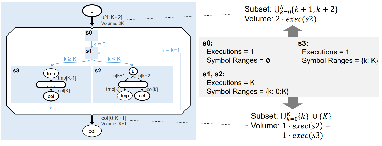
Fig. 8 Memlet propagation through a nested SDFG with a loop.
DaCe uses the SymPy symbolic engine to perform this projection, as well as to union
multiple internal memlets for propagation. The projection is performed in the propagation module, using
pattern matching on symbolic expressions. The MemletPattern class is used to define
such patterns, and the function propagate_subset() performs the propagation itself.
The process is triggered automatically by the Python frontend. If you want to trigger it manually on an entire SDFG, call
propagate_memlets_sdfg(). Note, however, that this may be a slow process depending on the
size of the SDFG. To propagate a single memlet, use propagate_memlet(), and for a single scope
use propagate_memlets_scope(). If you only want to trigger the part that propagates
symbol values across the SDFG state machine, call propagate_states().
SDFG Builder API
When writing frontends for DaCe and when transforming SDFGs, it is necessary to interact with the SDFG directly. The SDFG builder API provides a set of functions that allow the user to create SDFGs programmatically. The API is similar to graph manipulation APIs, such as NetworkX (in fact, the SDFG is internally represented as an ordered NetworkX graph).
The entire API is organized around methods of the SDFG and SDFGState
classes. Additionally, helper functions in dace.sdfg.utils and dace.transformation.helpers can be used
to perform common operations, such as traversal, querying, analysis, graph nesting, and many others.
Adding/removing elements: The two classes contain add_* methods for adding nodes and edges, and remove_* methods for
removing them. Examples include add_tasklet() and add_edge().
Other helper methods can compose these operations, such as add_mapped_tasklet(), which adds
a tasklet inside a map; and add_memlet_path() which adds a path of memlets between an
arbitrary number of scopes, propagating them along the way.
Connectors and edges: The methods add_{in,out}_connector on subclasses of Node add
appropriate connectors (view or passthrough) to the node. The add_edge() method of
SDFGState receives two nodes and two connector names, and creates an edge between them.
add_nedge() (no-connector edge) acts as a shorthand for edges with
None connectors on either side.
Enumeration: The API can enumerate the specific nodes and edges of a graph via the nodes() and edges() methods.
The interface also contains methods for querying the graph, such as all_nodes_recursive(), which is
useful to obtain all nodes, including states and nodes of nested SDFGs (similarly, all_edges_recursive()
and all_sdfgs_recursive() query edges and SDFGs, respectively). Navigating within states can
be performed using the scope methods.
Subgraphs: The API allows the user to obtain subgraphs of the SDFG, such as the scope_subgraph()
method, which returns a subgraph of the state that contains all nodes within a given scope. In general, the
SubgraphView class can be used to obtain a view of a subgraph. It filters out nodes and edges
that are not part of the subgraph, and can be used to perform operations on the subgraph, such as traversing it.
Data descriptors: Methods such as add_array() and add_stream()
can be used to add data descriptors to the SDFG. Any subclass of the Data base class
can be added to the SDFG using the add_datadesc() method.
Traversal: Since nodes and edges are stored in arbitrary order, the API provides methods for traversing the graph
by topological order. The method dfs_topological_sort() returns a list of nodes in a state, and
blockorder_topological_sort() traverses the state machine in approximate order of execution
(i.e., preserving order and entering if/for scopes before continuing).
What to Avoid
While SDFGs are Turing complete, they are not meant to be used to represent any program concisely.
Concepts such as parametric-depth recursion are control-centric (and not very portable). In order to represent them, a stack would need to be simulated in the representation, which will be slow. The frontends avoid parametric-depth recursion by creating a callback to the original runtime (e.g., the Python interpreter) instead of parsing it into an SDFG.
Another example is dynamic memory. Dynamically-allocated arrays are supported, so long as their sizes can be expressed as symbolic expressions. However, this would create another state in the state machine (see the example in Symbols), which might hamper dataflow analysis. In general, it is better to use constant or symbolically-sized memory allocation.
Lastly, complex pointer arithmetic and referencing different types of arrays with the same Reference are not supported. Frontends will try to mitigate this by creating multiple Reference data descriptors, but references in general inhibit provenance tracking of arrays, and many optimizations would not apply.
In many of the above cases, the frontends will emit a warning to the user, and unsupported behavior will be encapsulated as callbacks. It is important to pay attention to these warnings, as they might contribute to performance issues later on.
.sdfg File Format
An SDFG file is a JSON file that contains all the properties of the graph’s elements. See Properties and Serialization for more information about how those are saved.
You can save an SDFG to a file in the SDFG API with the save() method. Loading an SDFG from a
file uses the from_file() static method. For example, in the following save/load roundtrip:
@dace.program
def example(a: dace.float64[20]):
    return a + 1
sdfg = example.to_sdfg()  # Create an SDFG out of the DaCe program

sdfg.save('myfile.sdfg')  # Save
new_sdfg = dace.SDFG.from_file('myfile.sdfg')  # Reload

assert sdfg.hash_sdfg() == new_sdfg.hash_sdfg()  # OK, SDFGs are the same
The compress argument can be used to save a smaller (gzip compressed) file. It can keep the same extension,
but it is customary to use .sdfg.gz or .sdfgz to let others know it is compressed.
It is recommended to use this option for large SDFGs, as it not only saves space, but also speeds up loading and
editing of the SDFG in visualization tools and the VSCode extension.